TREX allows to assimilate, process and analyse sap flow data obtained with the thermal dissipation method (TDM). The package includes functions for gap filling time-series data, detecting outliers, calculating data-processing uncertainties and generating uniform data output and visualisation. The package is designed to deal with large quantities of data and apply commonly used data-processing methods. The functions have been validated on data collected from different tree species across the northern hemisphere (Peters et al. 2018 <doi: 10.1111/nph.15241>), and an accompanying manuscript has been published in Methods in Ecology and Evolution as (Peters et al. 2020 <doi: 10.1111/2041-210X.13524>)
1. Installation
The latest version of TREX can be installed and used via
If you want to use CRAN, we have a stable release version used for the MEE manuscript available named TREXr:
install.packages("TREXr")2. Basic use and workflow
Load data
# load raw data
raw   <- is.trex(example.data(type="doy"),
                 tz="GMT",
                 time.format="%H:%M",
                 solar.time=TRUE,
                 long.deg=7.7459,
                 ref.add=FALSE)

# adjust time steps
input <- dt.steps(input=raw,
                start="2013-05-01 00:00",
                end="2013-11-01 00:00",
                time.int=15,
                max.gap=60,
                decimals=10,
                df=FALSE)

# remove obvious outliers
input[which(input<0.2)]<- NA
Calculate maximum ΔT-Values
Three methods can be applied to calculate ΔT (or ΔV for voltage differences between TDM probes):
-
pd: pre-dawn -
mw: moving-window -
dr: double-regression
input <- tdm_dt.max(input,
                    methods = c("pd", "mw", "dr"),
                    det.pd = TRUE,
                    interpolate = FALSE,
                    max.days = 10,
                    df = FALSE)

plot(input$input, ylab = expression(Delta*italic("V")))

lines(input$max.pd, col = "green")
lines(input$max.mw, col = "blue")
lines(input$max.dr, col = "orange")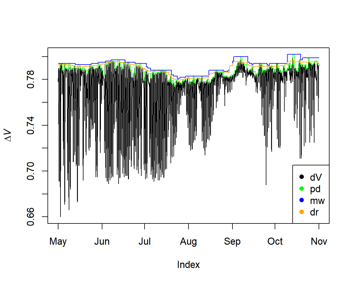
Calculate Sap Flux Density
output.data<- tdm_cal.sfd(input,make.plot=TRUE,df=FALSE,wood="Coniferous")

plot(output.data$sfd.pd$sfd[1:1000, ], ylim=c(0,10))
# see estimated uncertainty
lines(output.data$sfd.pd$q025[1:1000, ], lty=1,col="grey")
lines(output.data$sfd.pd$q975[1:1000, ], lty=1,col="grey")
lines(output.data$sfd.pd$sfd[1:1000, ])

sfd_data <- output.data$sfd.dr$sfd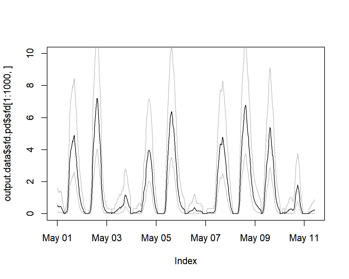
Generate Outputs
Here we generate outputs based on environmental filters and calculate crown conductance (Gc) values.
output<- out.data(input=sfd_data,
                  vpd.input=vpd,
                  sr.input=sr,
                  prec.input=preci,
                  low.sr = 150,
                  peak.sr=300,
                  vpd.cutoff= 0.5,
                  prec.lim=1,
                  method="env.filt",
                  max.quant=0.99,
                  make.plot=TRUE)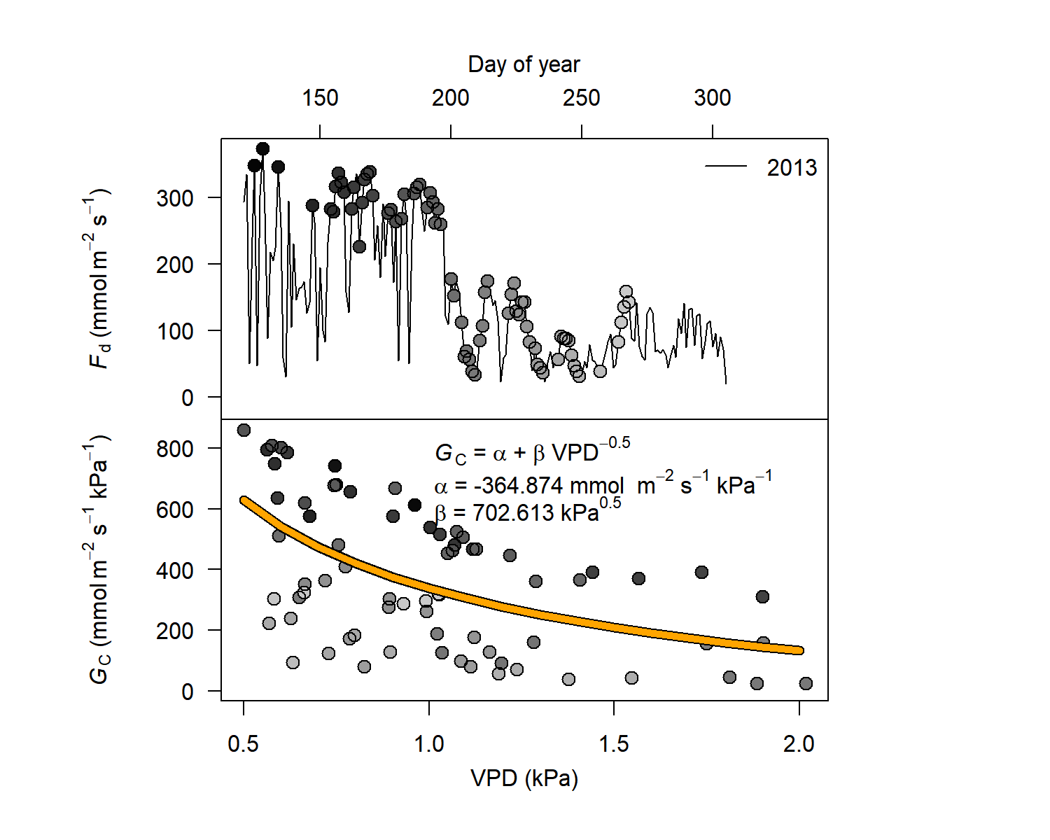
3. More on TREX
Workshops using TREX
-
ESA 2020:
TREXwas introduced and demonstrated in detail in a workshop during the Ecological Society of America’s 2020 AGM. The workshop description can be found here, and all materials on the dedicated page.
4. Citing this work
Please cite TREX when you apply it in your own work as:
Peters, RL, Pappas, C, Hurley, AG, et al. Assimilate, process and analyse thermal dissipation sap flow data using the TREX r package. Methods Ecol Evol. 2021; 12: 342– 350. https://doi.org/10.1111/2041-210X.13524
A reference is available in R using: