remis uses the UNFCCC Data Interface Flexible Query API
to download Inventory Data. At a later stage, functions for downloading
Compilation and Accounting Data (cad and
cadCP2) will be included.
Data downloads via queries require a variable for a specific party and
year, which are referred to via unique id’s. While party
and year id’s are linked to respective data in a fairly
straight-forward manner (e.g., single country or year), variable ids are
unique descriptors for a combination of data sources consisting of:
- category
- classification
- measurement
- gas
- unit
The above are referred to as ccmgu’s.
Initializing remis with rem_init provides a
list with several objects to inspect available data and query for it.
These include id overviews for parties, years,
ccmgu’s, as well as respective variable tables and the query
object for requests .req.
library(remis)
library(dplyr)
#>
#> Attaching package: 'dplyr'
#> The following objects are masked from 'package:stats':
#>
#>     filter, lag
#> The following objects are masked from 'package:base':
#>
#>     intersect, setdiff, setequal, union

rem <- rem_init()
#> parsing api/parties/
#> parsing api/years/single
#> parsing api/dimension-instances/category
#> parsing api/dimension-instances/classification
#> parsing api/dimension-instances/measure
#> parsing api/dimension-instances/gas
#> parsing api/conversion/fq
#> parsing api/variables/fq/annexOne
#> parsing api/variables/fq/nonAnnexOne

names(rem)
#>  [1] "parties"               "years"                 "categories"
#>  [4] "classification"        "measures"              "gas"
#>  [7] "units"                 "variables"             "duplicate_variableIds"
#> [10] ".req"
Note that only calls using the Flexible Query API are currently implemented. These allow interacting with data sources from:
- annexOne
- nonAnnexOne
- extData
Queries for data within cad and cadCP2 will be available in future versions.
Further details on the objects within rem are:
- parties - class: data.frame
- years - class: list
- categories - class: list
- classification - class: list
- measures - class: list
- gas - class: list
- units - class: list
- variables - class: list
- duplicate_variableIds - class: integer
- .req - class: HttpClient, R6
Building up Flexible Queries
Details on the Flexible Query API can be found in the official documentation of the Data Interface for UNFCCC.
Define whether annexOne or nonAnnexOne data shall be downloaded, and then:
- Select party
- Select year
- Choose variable based on
ccmgu’s - Execute query
Note, that objects in rem (excluding
parties) provide all data sources (where applicable)
reflected in the list items annexOne, nonAnnexOne, extData, cad,
cadCP2.
Example A
1. Select Party
Here we choose Germany and France.
# in RStudio:
# View(rem$parties)

parties_mask <- rem$parties$parties_code %in% c('DEU', 'FRA')
parties <- rem$parties[parties_mask, c('id', 'name', 'categoryCode')]
parties
#>    id    name categoryCode
#> 18 23  France     annexOne
#> 19 13 Germany     annexOne
Note, that both parties are in Annex I.
2. Select years
We will select all years from 1990 to the latest inventory year (2020).
# base year has id = 0
years <- rem$years$annexOne[rem$years$annexOne$id != 0, ]
years
#>    id                       name
#> 2  32                       1990
#> 3  33                       1991
#> 4  34                       1992
#> 5  35                       1993
#> 6  36                       1994
#> 7  37                       1995
#> 8  38                       1996
#> 9  39                       1997
#> 10 40                       1998
#> 11 41                       1999
#> 12 42                       2000
#> 13 43                       2001
#> 14 44                       2002
#> 15 45                       2003
#> 16 46                       2004
#> 17 47                       2005
#> 18 48                       2006
#> 19 49                       2007
#> 20 50                       2008
#> 21 51                       2009
#> 22 52                       2010
#> 23 53                       2011
#> 24 54                       2012
#> 25 55                       2013
#> 26 56                       2014
#> 27 57                       2015
#> 28 58                       2016
#> 29 59                       2017
#> 30 60                       2018
#> 31 61                       2019
#> 32 62 Last Inventory Year (2020)
3. Select from ccmug’s
The selection of ccmug’s is possible is several ways.
Ideally, one item of interest should be selected, such as a category or
a measure, through which the appropriate variable for querying is
identified. This can be done either by browsing in RStudio
with View(rem) and using the interactive filter function,
or by searching programmatically. The example below shows the
latter.
Here, we assume an interest in emissions from cars in the transportation sector by fuel type and in total in the CRF-Category 1.A.3.b.i Cars (id = 9279). Therefore, we begin with category as our starting point.
# parties are annexOne, thus:

category_mask <- grepl('1.A.3.b.i  Cars', rem$categories$annexOne$name)
category <- rem$categories$annexOne[category_mask, ]
as.data.frame(t(category))
#>                                                V1
#> id                                           9279
#> level_1                                    Totals
#> level_2           Total GHG emissions with LULUCF
#> level_3                                1.  Energy
#> level_4 1.AA  Fuel Combustion - Sectoral approach
#> level_5                          1.A.3  Transport
#> level_6              1.A.3.b  Road Transportation
#> level_7                           1.A.3.b.i  Cars
#> level_8                                      <NA>
#> name                              1.A.3.b.i  Cars
The table above also highlights the nesting structure throughout the CRF-Category tree.
Next, find appropriate variables (i.e. combination of ccmug’s) that contain our category of interest.
variables <- select_varid(
  vars = rem$variables$annexOne,
  category_id = category$id)
head(variables, 20)
#>      variableId categoryId classificationId measureId gasId unitId
#> 1439      17578       9279            10510     10460 10468      5
#> 1451     924766       9279            10525     10460 10468      5
#> 1459     925785       9279            10530     10460 10471      5
#> 2406     924906       9279            10538     10460 10471      5
#> 2425     926628       9279            10525     10460 10469      5
#> 2730     926278       9279            10528     10460 10468      5
#> 2864     925125       9279            10530     10460 10468      5
#> 3019     924993       9279            10530     10460 10469      5
#> 3028     926280       9279            10528     10460 10471      5
#> 3887     926287       9279            10520     10460 10469      5
#> 4055     928586       9279            10525     10591 10469     28
#> 4096     928580       9279            10513     10591 10469     28
#> 4103     928626       9279            10524     10591 10469     28
#> 4105     928544       9279            10528     10591 10469     28
#> 4204     925435       9279            10538     10460 10468      5
#> 4205     925469       9279            10524     10460 10471      5
#> 4207     926637       9279            10520     10460 10468      5
#> 4229      94409       9279            10510     10460 10471      5
#> 4243     925496       9279            10513     10460 10468      5
#> 4254     925453       9279            10524     10460 10469      5
There are a total of 60 variable combinations that include our
category of interest. Note that select_varid() also allows
selections by including other ccmugs to be more specific.
Let’s inspect the variables in a more human-readable format:
variables_text <- get_variables(
  rms = rem,
  variable_id = variables$variableId)
variables_text[order(variables_text$classification, variables_text$measure), ]
#>    variableId      categoryId                classificationId
#> 43     927370 1.A.3.b.i  Cars                         Biomass
#> 48     928580 1.A.3.b.i  Cars                         Biomass
#> 56     928872 1.A.3.b.i  Cars                         Biomass
#> 58     928896 1.A.3.b.i  Cars                         Biomass
#> 4      200184 1.A.3.b.i  Cars                         Biomass
#> 21     925496 1.A.3.b.i  Cars                         Biomass
#> 32     926374 1.A.3.b.i  Cars                         Biomass
#> 33     926583 1.A.3.b.i  Cars                         Biomass
#> 44     927427 1.A.3.b.i  Cars                      Diesel Oil
#> 46     928524 1.A.3.b.i  Cars                      Diesel Oil
#> 57     928873 1.A.3.b.i  Cars                      Diesel Oil
#> 60     928966 1.A.3.b.i  Cars                      Diesel Oil
#> 5      200185 1.A.3.b.i  Cars                      Diesel Oil
#> 29     926287 1.A.3.b.i  Cars                      Diesel Oil
#> 35     926637 1.A.3.b.i  Cars                      Diesel Oil
#> 36     926785 1.A.3.b.i  Cars                      Diesel Oil
#> 42     927327 1.A.3.b.i  Cars                   Gaseous Fuels
#> 50     928626 1.A.3.b.i  Cars                   Gaseous Fuels
#> 51     928708 1.A.3.b.i  Cars                   Gaseous Fuels
#> 55     928864 1.A.3.b.i  Cars                   Gaseous Fuels
#> 6      200186 1.A.3.b.i  Cars                   Gaseous Fuels
#> 15     924937 1.A.3.b.i  Cars                   Gaseous Fuels
#> 19     925453 1.A.3.b.i  Cars                   Gaseous Fuels
#> 20     925469 1.A.3.b.i  Cars                   Gaseous Fuels
#> 45     927449 1.A.3.b.i  Cars                        Gasoline
#> 49     928586 1.A.3.b.i  Cars                        Gasoline
#> 54     928849 1.A.3.b.i  Cars                        Gasoline
#> 59     928909 1.A.3.b.i  Cars                        Gasoline
#> 7      200187 1.A.3.b.i  Cars                        Gasoline
#> 13     924766 1.A.3.b.i  Cars                        Gasoline
#> 26     926275 1.A.3.b.i  Cars                        Gasoline
#> 34     926628 1.A.3.b.i  Cars                        Gasoline
#> 38     927111 1.A.3.b.i  Cars Liquefied Petroleum Gases (LPG)
#> 47     928544 1.A.3.b.i  Cars Liquefied Petroleum Gases (LPG)
#> 52     928803 1.A.3.b.i  Cars Liquefied Petroleum Gases (LPG)
#> 53     928813 1.A.3.b.i  Cars Liquefied Petroleum Gases (LPG)
#> 8      200188 1.A.3.b.i  Cars Liquefied Petroleum Gases (LPG)
#> 27     926278 1.A.3.b.i  Cars Liquefied Petroleum Gases (LPG)
#> 28     926280 1.A.3.b.i  Cars Liquefied Petroleum Gases (LPG)
#> 31     926309 1.A.3.b.i  Cars Liquefied Petroleum Gases (LPG)
#> 39     927130 1.A.3.b.i  Cars                    Liquid Fuels
#> 9      200189 1.A.3.b.i  Cars                    Liquid Fuels
#> 16     924993 1.A.3.b.i  Cars                    Liquid Fuels
#> 17     925125 1.A.3.b.i  Cars                    Liquid Fuels
#> 23     925785 1.A.3.b.i  Cars                    Liquid Fuels
#> 40     927199 1.A.3.b.i  Cars              Other Fossil Fuels
#> 10     200190 1.A.3.b.i  Cars              Other Fossil Fuels
#> 14     924906 1.A.3.b.i  Cars              Other Fossil Fuels
#> 18     925435 1.A.3.b.i  Cars              Other Fossil Fuels
#> 22     925688 1.A.3.b.i  Cars              Other Fossil Fuels
#> 37     927097 1.A.3.b.i  Cars              Other Liquid Fuels
#> 11     200191 1.A.3.b.i  Cars              Other Liquid Fuels
#> 24     926080 1.A.3.b.i  Cars              Other Liquid Fuels
#> 25     926180 1.A.3.b.i  Cars              Other Liquid Fuels
#> 30     926297 1.A.3.b.i  Cars              Other Liquid Fuels
#> 41     927247 1.A.3.b.i  Cars              Total for category
#> 1       17578 1.A.3.b.i  Cars              Total for category
#> 2       94409 1.A.3.b.i  Cars              Total for category
#> 3      173310 1.A.3.b.i  Cars              Total for category
#> 12     715050 1.A.3.b.i  Cars              Total for category
#>                  measureId          gasId            unitId reporting
#> 43        Fuel Consumption         No gas                TJ  annexOne
#> 48 Implied emission factor            CO₂              t/TJ  annexOne
#> 56 Implied emission factor            N₂O             kg/TJ  annexOne
#> 58 Implied emission factor            CH₄             kg/TJ  annexOne
#> 4   Net emissions/removals Aggregate GHGs kt CO₂ equivalent  annexOne
#> 21  Net emissions/removals            CH₄                kt  annexOne
#> 32  Net emissions/removals            N₂O                kt  annexOne
#> 33  Net emissions/removals            CO₂                kt  annexOne
#> 44        Fuel Consumption         No gas                TJ  annexOne
#> 46 Implied emission factor            CO₂              t/TJ  annexOne
#> 57 Implied emission factor            N₂O             kg/TJ  annexOne
#> 60 Implied emission factor            CH₄             kg/TJ  annexOne
#> 5   Net emissions/removals Aggregate GHGs kt CO₂ equivalent  annexOne
#> 29  Net emissions/removals            CO₂                kt  annexOne
#> 35  Net emissions/removals            CH₄                kt  annexOne
#> 36  Net emissions/removals            N₂O                kt  annexOne
#> 42        Fuel Consumption         No gas                TJ  annexOne
#> 50 Implied emission factor            CO₂              t/TJ  annexOne
#> 51 Implied emission factor            N₂O             kg/TJ  annexOne
#> 55 Implied emission factor            CH₄             kg/TJ  annexOne
#> 6   Net emissions/removals Aggregate GHGs kt CO₂ equivalent  annexOne
#> 15  Net emissions/removals            CH₄                kt  annexOne
#> 19  Net emissions/removals            CO₂                kt  annexOne
#> 20  Net emissions/removals            N₂O                kt  annexOne
#> 45        Fuel Consumption         No gas                TJ  annexOne
#> 49 Implied emission factor            CO₂              t/TJ  annexOne
#> 54 Implied emission factor            N₂O             kg/TJ  annexOne
#> 59 Implied emission factor            CH₄             kg/TJ  annexOne
#> 7   Net emissions/removals Aggregate GHGs kt CO₂ equivalent  annexOne
#> 13  Net emissions/removals            CH₄                kt  annexOne
#> 26  Net emissions/removals            N₂O                kt  annexOne
#> 34  Net emissions/removals            CO₂                kt  annexOne
#> 38        Fuel Consumption         No gas                TJ  annexOne
#> 47 Implied emission factor            CO₂              t/TJ  annexOne
#> 52 Implied emission factor            CH₄             kg/TJ  annexOne
#> 53 Implied emission factor            N₂O             kg/TJ  annexOne
#> 8   Net emissions/removals Aggregate GHGs kt CO₂ equivalent  annexOne
#> 27  Net emissions/removals            CH₄                kt  annexOne
#> 28  Net emissions/removals            N₂O                kt  annexOne
#> 31  Net emissions/removals            CO₂                kt  annexOne
#> 39        Fuel Consumption         No gas                TJ  annexOne
#> 9   Net emissions/removals Aggregate GHGs kt CO₂ equivalent  annexOne
#> 16  Net emissions/removals            CO₂                kt  annexOne
#> 17  Net emissions/removals            CH₄                kt  annexOne
#> 23  Net emissions/removals            N₂O                kt  annexOne
#> 40        Fuel Consumption         No gas                TJ  annexOne
#> 10  Net emissions/removals Aggregate GHGs kt CO₂ equivalent  annexOne
#> 14  Net emissions/removals            N₂O                kt  annexOne
#> 18  Net emissions/removals            CH₄                kt  annexOne
#> 22  Net emissions/removals            CO₂                kt  annexOne
#> 37        Fuel Consumption         No gas                TJ  annexOne
#> 11  Net emissions/removals Aggregate GHGs kt CO₂ equivalent  annexOne
#> 24  Net emissions/removals            N₂O                kt  annexOne
#> 25  Net emissions/removals            CH₄                kt  annexOne
#> 30  Net emissions/removals            CO₂                kt  annexOne
#> 41        Fuel Consumption         No gas                TJ  annexOne
#> 1   Net emissions/removals            CH₄                kt  annexOne
#> 2   Net emissions/removals            N₂O                kt  annexOne
#> 3   Net emissions/removals            CO₂                kt  annexOne
#> 12  Net emissions/removals Aggregate GHGs kt CO₂ equivalent  annexOne
Next, we filter for the desired measure
Net emissions/removals and gas
Aggregate GHGs:
var_ids <- variables_text[variables_text$measure=="Net emissions/removals" &
                 variables_text$gas=="Aggregate GHGs", ]
var_ids
#>    variableId      categoryId                classificationId
#> 4      200184 1.A.3.b.i  Cars                         Biomass
#> 5      200185 1.A.3.b.i  Cars                      Diesel Oil
#> 6      200186 1.A.3.b.i  Cars                   Gaseous Fuels
#> 7      200187 1.A.3.b.i  Cars                        Gasoline
#> 8      200188 1.A.3.b.i  Cars Liquefied Petroleum Gases (LPG)
#> 9      200189 1.A.3.b.i  Cars                    Liquid Fuels
#> 10     200190 1.A.3.b.i  Cars              Other Fossil Fuels
#> 11     200191 1.A.3.b.i  Cars              Other Liquid Fuels
#> 12     715050 1.A.3.b.i  Cars              Total for category
#>                 measureId          gasId            unitId reporting
#> 4  Net emissions/removals Aggregate GHGs kt CO₂ equivalent  annexOne
#> 5  Net emissions/removals Aggregate GHGs kt CO₂ equivalent  annexOne
#> 6  Net emissions/removals Aggregate GHGs kt CO₂ equivalent  annexOne
#> 7  Net emissions/removals Aggregate GHGs kt CO₂ equivalent  annexOne
#> 8  Net emissions/removals Aggregate GHGs kt CO₂ equivalent  annexOne
#> 9  Net emissions/removals Aggregate GHGs kt CO₂ equivalent  annexOne
#> 10 Net emissions/removals Aggregate GHGs kt CO₂ equivalent  annexOne
#> 11 Net emissions/removals Aggregate GHGs kt CO₂ equivalent  annexOne
#> 12 Net emissions/removals Aggregate GHGs kt CO₂ equivalent  annexOne
All relevant information (e.g., units, type of gas) are provided
here. In addition, unit conversion factors can be identified by looking
up relevant source and target units in rem$units$units and
cross-referencing them in rem$units$annexOne.
4. Query for download
Queries using the Flexible Query API are done
flex_query(), which uses the .req object in
rem to make a POST request:
result <- flex_query(
  rem,
  variable_ids = var_ids$variableId,
  party_ids = parties$id,
  year_ids = years$id,
  pretty = TRUE)

head(result, 20)
#>    parties years variableId      categoryId classificationId
#> 1  Germany  1990     200184 1.A.3.b.i  Cars          Biomass
#> 2  Germany  1991     200184 1.A.3.b.i  Cars          Biomass
#> 3  Germany  1992     200184 1.A.3.b.i  Cars          Biomass
#> 4  Germany  1993     200184 1.A.3.b.i  Cars          Biomass
#> 5  Germany  1994     200184 1.A.3.b.i  Cars          Biomass
#> 6  Germany  1995     200184 1.A.3.b.i  Cars          Biomass
#> 7  Germany  1996     200184 1.A.3.b.i  Cars          Biomass
#> 8  Germany  1997     200184 1.A.3.b.i  Cars          Biomass
#> 9  Germany  1998     200184 1.A.3.b.i  Cars          Biomass
#> 10 Germany  1999     200184 1.A.3.b.i  Cars          Biomass
#> 11 Germany  2000     200184 1.A.3.b.i  Cars          Biomass
#> 12 Germany  2001     200184 1.A.3.b.i  Cars          Biomass
#> 13 Germany  2002     200184 1.A.3.b.i  Cars          Biomass
#> 14 Germany  2003     200184 1.A.3.b.i  Cars          Biomass
#> 15 Germany  2004     200184 1.A.3.b.i  Cars          Biomass
#> 16 Germany  2005     200184 1.A.3.b.i  Cars          Biomass
#> 17 Germany  2006     200184 1.A.3.b.i  Cars          Biomass
#> 18 Germany  2007     200184 1.A.3.b.i  Cars          Biomass
#> 19 Germany  2008     200184 1.A.3.b.i  Cars          Biomass
#> 20 Germany  2009     200184 1.A.3.b.i  Cars          Biomass
#>                 measureId          gasId            unitId reporting
#> 1  Net emissions/removals Aggregate GHGs kt CO₂ equivalent  annexOne
#> 2  Net emissions/removals Aggregate GHGs kt CO₂ equivalent  annexOne
#> 3  Net emissions/removals Aggregate GHGs kt CO₂ equivalent  annexOne
#> 4  Net emissions/removals Aggregate GHGs kt CO₂ equivalent  annexOne
#> 5  Net emissions/removals Aggregate GHGs kt CO₂ equivalent  annexOne
#> 6  Net emissions/removals Aggregate GHGs kt CO₂ equivalent  annexOne
#> 7  Net emissions/removals Aggregate GHGs kt CO₂ equivalent  annexOne
#> 8  Net emissions/removals Aggregate GHGs kt CO₂ equivalent  annexOne
#> 9  Net emissions/removals Aggregate GHGs kt CO₂ equivalent  annexOne
#> 10 Net emissions/removals Aggregate GHGs kt CO₂ equivalent  annexOne
#> 11 Net emissions/removals Aggregate GHGs kt CO₂ equivalent  annexOne
#> 12 Net emissions/removals Aggregate GHGs kt CO₂ equivalent  annexOne
#> 13 Net emissions/removals Aggregate GHGs kt CO₂ equivalent  annexOne
#> 14 Net emissions/removals Aggregate GHGs kt CO₂ equivalent  annexOne
#> 15 Net emissions/removals Aggregate GHGs kt CO₂ equivalent  annexOne
#> 16 Net emissions/removals Aggregate GHGs kt CO₂ equivalent  annexOne
#> 17 Net emissions/removals Aggregate GHGs kt CO₂ equivalent  annexOne
#> 18 Net emissions/removals Aggregate GHGs kt CO₂ equivalent  annexOne
#> 19 Net emissions/removals Aggregate GHGs kt CO₂ equivalent  annexOne
#> 20 Net emissions/removals Aggregate GHGs kt CO₂ equivalent  annexOne
#>    number_value string_value
#> 1            NA           NA
#> 2            NA           NA
#> 3            NA           NA
#> 4            NA           NA
#> 5            NA           NA
#> 6      33.78233         <NA>
#> 7      46.03468         <NA>
#> 8      79.19863         <NA>
#> 9      82.90973         <NA>
#> 10    109.39233         <NA>
#> 11    261.02488         <NA>
#> 12    389.07220         <NA>
#> 13    512.62435         <NA>
#> 14    793.73382         <NA>
#> 15   1193.50417         <NA>
#> 16   2614.46296         <NA>
#> 17   4668.01095         <NA>
#> 18   5080.86875         <NA>
#> 19   4435.05037         <NA>
#> 20   4446.86238         <NA>
See results:
library(ggplot2)
result %>%
  setNames(nm = gsub("Id", "", names(.))) %>%
  mutate(years = as.numeric(gsub('[^0-9]', "", result$years, perl = TRUE))) %>%
  ggplot(aes(x = years, y = number_value, color = parties)) +
  geom_line() +
  facet_wrap(~classification, scales = "free_y") +
  labs(y = sprintf('GHG-Emissions [%s]', unique(result$unit)),
       title = unique(result$category)) +
  theme_minimal(base_size = 16) +
  theme(legend.position = 'top', legend.direction = 'horizontal')
#> Warning: Removed 7 rows containing missing values (`geom_line()`).![]()
`%nin%` <- Negate(`%in%`)

result %>%
  setNames(nm = gsub("Id", "", names(.))) %>%
  mutate(years = as.numeric(gsub('[^0-9]', "", years, perl = TRUE))) %>%
  filter(classification %nin% c('Total for category', 'Gaseous Fuels', 'Liquid Fuels')) %>%
  group_by(parties, years) %>%
  mutate(percent_contribution = number_value/sum(number_value, na.rm = TRUE) * 100,
            ) %>%
  ggplot(aes(y = as.factor(years), x = percent_contribution, fill = classification)) +
  geom_bar(stat = 'identity') +
  facet_wrap(~parties) +
  labs(x = 'Contribution [%]',
       y = 'Year',
       title = unique(result$category)) +
  theme_minimal(base_size = 16) +
  scale_fill_brewer(palette = 'Set2', direction = -1)
#> Warning: Removed 76 rows containing missing values (`position_stack()`).![]()
Example B
Here we will exploit the Flexible Queries API to download
extData, focusing on the World Bank population data.
#> # A tibble: 4 × 4
#>      id level_1       level_2                      name
#>   <int> <chr>         <chr>                        <chr>
#> 1 10501 External Data NA                           External Data
#> 2 10502 External Data Country Area                 Country Area
#> 3 10503 External Data Gross Domestic Product - GDP Gross Domestic Product - GDP
#> 4 10504 External Data Population                   Population
# from extData - select Population Category:
category_mask <- grepl('Population', rem$categories$extData$name, fixed = FALSE)
category <- rem$categories$extData[category_mask, ]

# find variableIds containing population - ensure appropriate annex category
# is used here based on desired party
var_ids <- select_varid(vars = rem$variables$annexOne, category_id = category$id)

# check and confirm desired variable is correct
get_variables(rms = rem, var_ids$variableId)
#>   variableId categoryId   classificationId        measureId  gasId    unitId
#> 1     188991 Population Total for category Total population No gas thousands
#>   reporting
#> 1   extData

population <- flex_query(
  rms = rem,
  variable_ids = var_ids$variableId,
  party_ids = parties$id,
  year_ids = years$id)
#> Warning in duplicate_check(rms, variable_id = variable_ids): Found duplicated variableId ids: 188991.
#>  Check results and possibly exclude unwanted observations.


population %>%
  setNames(nm = gsub("Id", "", names(.))) %>%
  mutate(years = as.numeric(gsub('[^0-9]', "", years, perl = TRUE))) %>%
  ggplot(aes(x = years, y = number_value, color = parties)) +
  geom_line(linewidth = 1.5) +
  labs(y = sprintf('Population [%s]', unique(population$unit)),
       title = unique(population$category)) +
  theme_minimal(base_size = 16) +
  theme(legend.position = 'top', legend.direction = 'horizontal')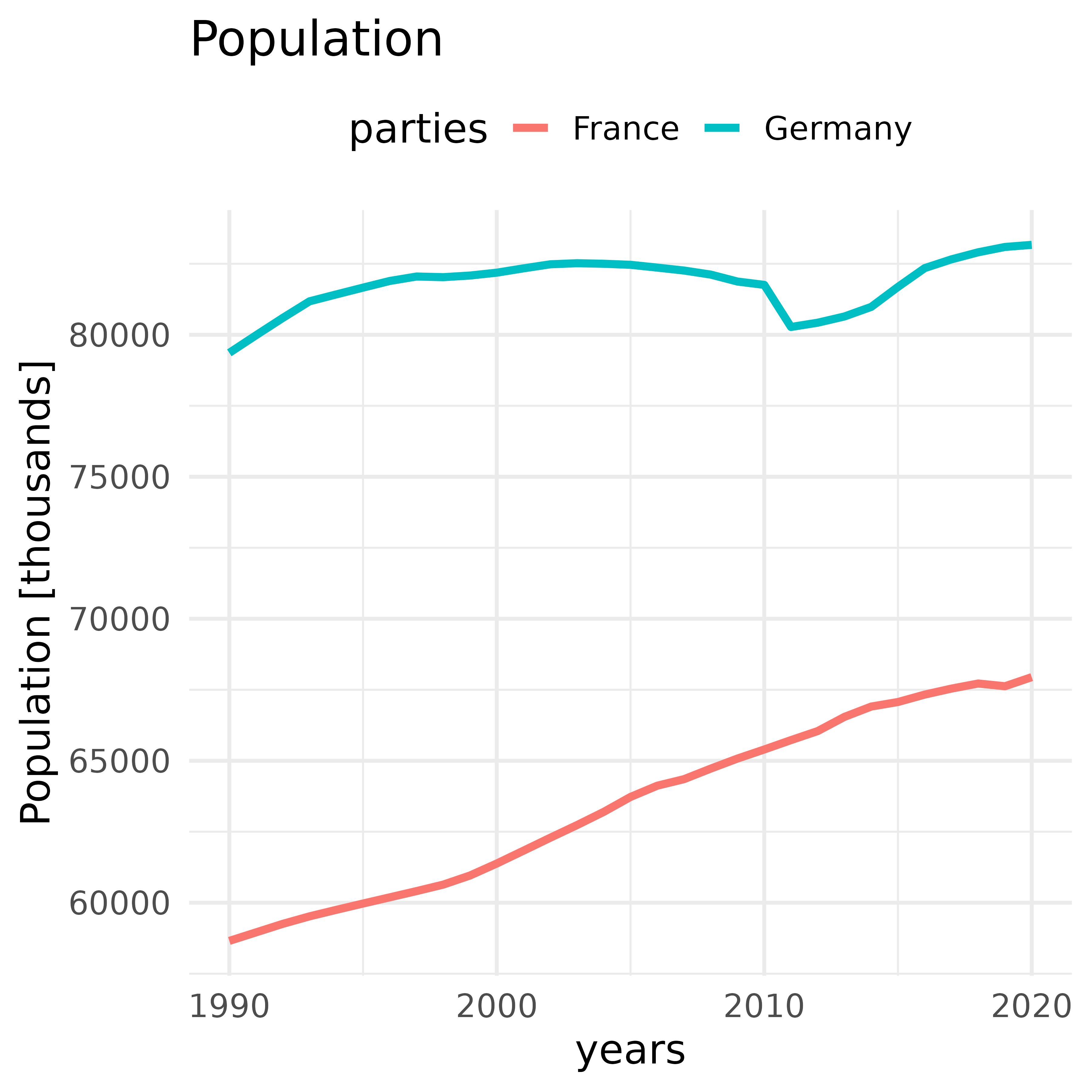
Example C
The code below downloads and visualizes a time series which was used in a decomposition analyses in the Biennial Report of the Expert Council on Climate Change issues, as given in Table 4, p. 220. The data is from Table1.A(a)s1 of the National Inventory Report after UNFCCC, CRF-Category 1.A.1.a Public Electricity and Heat Production.
# check
cat1A1a <- rem$categories$annexOne[grepl("1.A.1.a.", rem$categories$annexOne$name), ]

# manually choose id
# cat1A1a$id[1]

# get variables
cat1A1a_variables <- get_variables(
  rms = rem,
  select_varid(vars = rem$variables$annexOne, cat1A1a$id[1])$variableId
)

#choose id:
var_id <- cat1A1a_variables %>%
  filter(classificationId == 'Total for category',
         gasId == 'Aggregate GHGs'
  ) %>%
  dplyr::glimpse() %>%
  dplyr::pull(variableId)
#> Rows: 1
#> Columns: 7
#> $ variableId       <int> 714972
#> $ categoryId       <chr> "1.A.1.a  Public Electricity and Heat Production"
#> $ classificationId <chr> "Total for category"
#> $ measureId        <chr> "Net emissions/removals"
#> $ gasId            <chr> "Aggregate GHGs"
#> $ unitId           <chr> "kt CO₂ equivalent"
#> $ reporting        <chr> "annexOne"

# download data
cat1A1a_agg_ghg <- flex_query(
  rms = rem,
  variable_ids = var_id,
  party_ids = 13,
  year_ids = rem$years$annexOne$id)

# data includes year = "base year",
# for most parties this = 1990, but may vary.
# the code below replaces 'Base year' with NA, and thus discards the observation.
# see UNFCCC API documentation
cat1A1a_agg_ghg %>%
  mutate(years = as.numeric(gsub('[^0-9]', "", years, perl = TRUE))) %>%
  ggplot(aes(x = years, y = number_value)) +
  geom_line(linewidth = 1, color = 'steelblue') +
  geom_point(color = 'steelblue', size = 3) +
  labs(y = sprintf('GHG-Emissions [%s]', unique(cat1A1a_agg_ghg$unitId)),
       title = unique(cat1A1a_agg_ghg$categoryId)) +
  theme_minimal(base_size = 16) +
  theme(legend.position = 'top', legend.direction = 'horizontal')
#> Warning: Removed 1 row containing missing values (`geom_line()`).
#> Warning: Removed 1 rows containing missing values (`geom_point()`).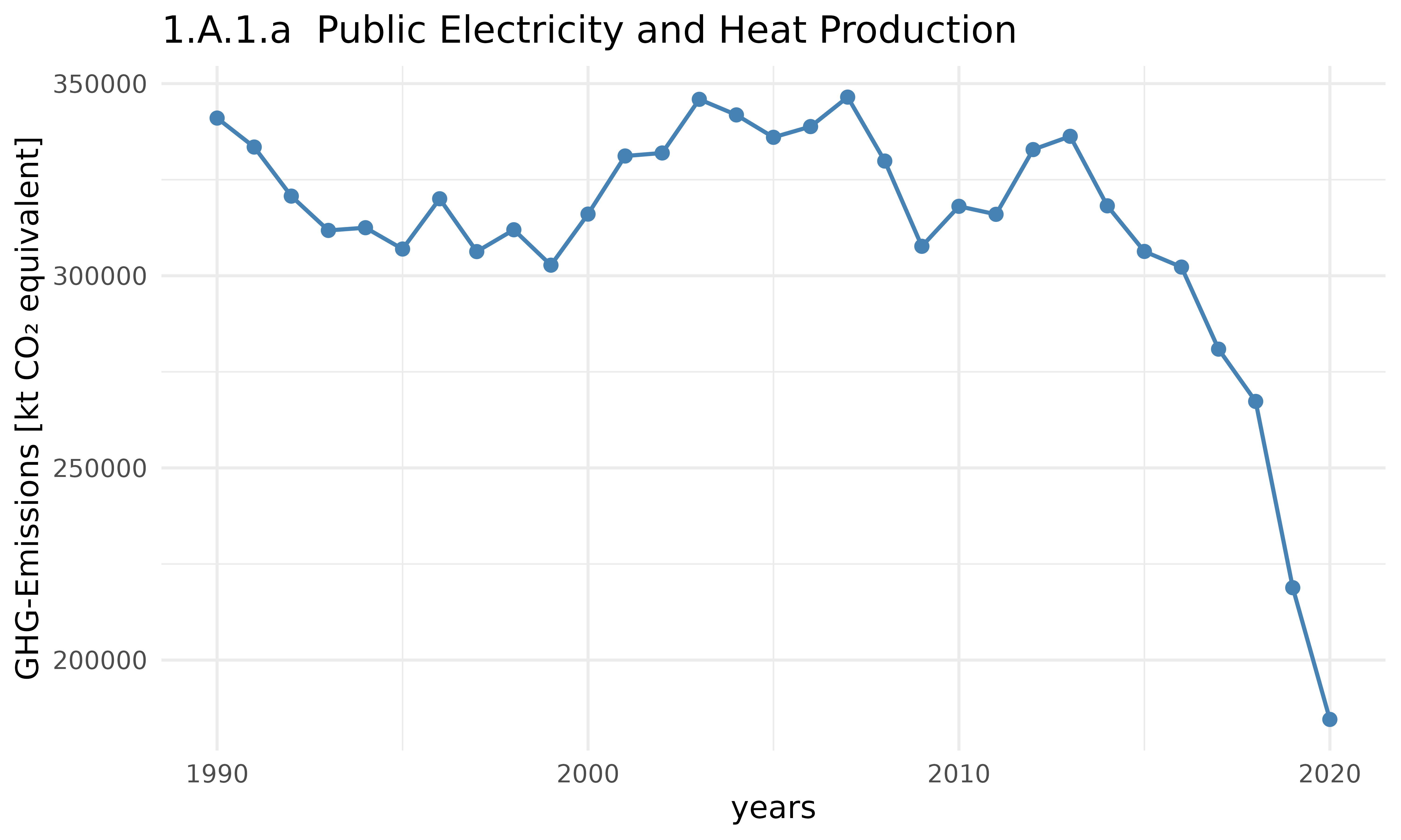
Duplicates
There are several duplicate variable id’s in the UNFCCC DI (n = 360).
Duplicated variables seem to only differ in one ccmug and have
the identical number / string value. Duplicated variables are listed in
rem$duplicated_variableIds.
For example:
rem$variables$annexOne[rem$variables$annexOne$variableId == rem$duplicate_variableIds[2], ]
#>     variableId categoryId classificationId measureId gasId unitId
#> 440     170726       8465            10510     10460 10471      5
#> 441     170726       8465            10820     10460 10471      5

get_variables(
  rem,
  rem$variables$annexOne[
    rem$variables$annexOne$variableId == rem$duplicate_variableIds[2],
    ]$variableId)
#>   variableId                                 categoryId
#> 1     170726 4.E.2.d  Wetlands Converted to Settlements
#> 2     170726 4.E.2.d  Wetlands Converted to Settlements
#>                                                     classificationId
#> 1                                                 Total for category
#> 2 4 (III) Direct N2O Emissions from N Mineralization/ Immobilization
#>                measureId gasId unitId reporting
#> 1 Net emissions/removals   N₂O     kt  annexOne
#> 2 Net emissions/removals   N₂O     kt  annexOne
Meta Overview
Parties
Parties are stored in rem$parties
# up to 5th entry on parties
knitr::kable(rem$parties %>%
               dplyr::group_by(name_code) %>%
dplyr::slice(1:3))| name_code | categoryCode | id | parties_code | name | parties_noData |
|---|---|---|---|---|---|
| Annex I | annexOne | 3 | AUS | Australia | NA |
| Annex I | annexOne | 4 | AUT | Austria | NA |
| Annex I | annexOne | 7 | BLR | Belarus | NA |
| Groups | annexOne | 1000001 | ANI | Annex I | NA |
| Groups | annexOne | 1000002 | ANEIT | Annex I EIT | NA |
| Groups | annexOne | 1000003 | ANNEIT | Annex I non-EIT | NA |
| Non Annex I | nonAnnexOne | 100064 | AFG | Afghanistan | NA |
| Non Annex I | nonAnnexOne | 100065 | ALB | Albania | NA |
| Non Annex I | nonAnnexOne | 100066 | DZA | Algeria | NA |
Years
Years are stored in rem$years for respective
| x |
|---|
| annexOne |
| nonAnnexOne |
| cad |
| cadCP2 |
knitr::kable(rem$years$annexOne)| id | name |
|---|---|
| 0 | Base year |
| 32 | 1990 |
| 33 | 1991 |
| 34 | 1992 |
| 35 | 1993 |
| 36 | 1994 |
| 37 | 1995 |
| 38 | 1996 |
| 39 | 1997 |
| 40 | 1998 |
| 41 | 1999 |
| 42 | 2000 |
| 43 | 2001 |
| 44 | 2002 |
| 45 | 2003 |
| 46 | 2004 |
| 47 | 2005 |
| 48 | 2006 |
| 49 | 2007 |
| 50 | 2008 |
| 51 | 2009 |
| 52 | 2010 |
| 53 | 2011 |
| 54 | 2012 |
| 55 | 2013 |
| 56 | 2014 |
| 57 | 2015 |
| 58 | 2016 |
| 59 | 2017 |
| 60 | 2018 |
| 61 | 2019 |
| 62 | Last Inventory Year (2020) |
Variable Overview (ccmug)
Sections below give a brief overview on ccmgu’s.
Categories
Categories are UNFCCC CRF-Categories or categories under the
Compilation and Accounting Data. The tables for each category have an
id and a name column. Where nested
sub-categories exist, additional columns using the name
level_x (x = nesting depth) show the category
hierarchy.
| x |
|---|
| annexOne |
| nonAnnexOne |
| extData |
| cad |
| cadCP2 |
| id | level_1 | level_2 | level_3 | level_4 | level_5 | level_6 | level_7 | level_8 | name |
|---|---|---|---|---|---|---|---|---|---|
| 10465 | Totals | NA | NA | NA | NA | NA | NA | NA | Totals |
| 10479 | Totals | Total GHG emissions without LULUCF including indirect CO₂ | NA | NA | NA | NA | NA | NA | Total GHG emissions without LULUCF including indirect CO₂ |
| 10480 | Totals | Total GHG emissions with LULUCF including indirect CO₂ | NA | NA | NA | NA | NA | NA | Total GHG emissions with LULUCF including indirect CO₂ |
| 10464 | Totals | Total GHG emissions without LULUCF | NA | NA | NA | NA | NA | NA | Total GHG emissions without LULUCF |
| 8677 | Totals | Total GHG emissions with LULUCF | NA | NA | NA | NA | NA | NA | Total GHG emissions with LULUCF |
| 10481 | Totals | Total GHG emissions without LULUCF | 1. Energy | NA | NA | NA | NA | NA | 1. Energy |
| 10482 | Totals | Total GHG emissions without LULUCF | 2. Industrial Processes and Product Use | NA | NA | NA | NA | NA | 2. Industrial Processes and Product Use |
| 10483 | Totals | Total GHG emissions without LULUCF | 3. Agriculture | NA | NA | NA | NA | NA | 3. Agriculture |
| 10484 | Totals | Total GHG emissions without LULUCF | 5. Waste | NA | NA | NA | NA | NA | 5. Waste |
| 10485 | Totals | Total GHG emissions without LULUCF | 6. Other | NA | NA | NA | NA | NA | 6. Other |
| id | level_1 | level_2 | level_3 | level_4 | level_5 | level_6 | level_7 | level_8 | name |
|---|---|---|---|---|---|---|---|---|---|
| 9116 | Totals | Total GHG emissions with LULUCF | 1. Energy | 1.B Fugitive Emissions from Fuels | 1.B.1 Solid Fuels | 1.B.1.a Coal Mining and Handling | 1.B.1.a.i Underground Mines | NA | 1.B.1.a.i Underground Mines |
| 8573 | Totals | Total GHG emissions with LULUCF | 1. Energy | 1.B Fugitive Emissions from Fuels | 1.B.1 Solid Fuels | 1.B.1.a Coal Mining and Handling | 1.B.1.a.ii Surface Mines | NA | 1.B.1.a.ii Surface Mines |
| 9933 | Totals | Total GHG emissions with LULUCF | 1. Energy | 1.B Fugitive Emissions from Fuels | 1.B.1 Solid Fuels | 1.B.1.a Coal Mining and Handling | 1.B.1.a.i Underground Mines | 1.B.1.a.i.1 Mining Activities | 1.B.1.a.i.1 Mining Activities |
| 9427 | Totals | Total GHG emissions with LULUCF | 1. Energy | 1.B Fugitive Emissions from Fuels | 1.B.1 Solid Fuels | 1.B.1.a Coal Mining and Handling | 1.B.1.a.i Underground Mines | 1.B.1.a.i.2 Post-Mining Activities | 1.B.1.a.i.2 Post-Mining Activities |
| 8211 | Totals | Total GHG emissions with LULUCF | 1. Energy | 1.B Fugitive Emissions from Fuels | 1.B.1 Solid Fuels | 1.B.1.a Coal Mining and Handling | 1.B.1.a.i Underground Mines | 1.B.1.a.i.3 Abandoned Underground Mines | 1.B.1.a.i.3 Abandoned Underground Mines |
| 10282 | Totals | Total GHG emissions with LULUCF | 1. Energy | 1.B Fugitive Emissions from Fuels | 1.B.1 Solid Fuels | 1.B.1.a Coal Mining and Handling | 1.B.1.a.ii Surface Mines | 1.B.1.a.ii.1 Mining Activities | 1.B.1.a.ii.1 Mining Activities |
| 9601 | Totals | Total GHG emissions with LULUCF | 1. Energy | 1.B Fugitive Emissions from Fuels | 1.B.1 Solid Fuels | 1.B.1.a Coal Mining and Handling | 1.B.1.a.ii Surface Mines | 1.B.1.a.ii.2 Post-Mining Activities | 1.B.1.a.ii.2 Post-Mining Activities |
Classification
Classification differ based on respective sectors and/or CRF-Categories:
- Energy:
- Fuel Types
- Agriculture:
- Livestock types
- LULUCF/LUCF:
- LULUCF/LUCF activities
| id | name |
|---|---|
| 10510 | Total for category |
| 10511 | Anthracite |
| 10512 | Aviation Gasoline |
| 10513 | Biomass |
| 10514 | Bitumen |
| 10515 | BKB and Patent Fuel |
| 10516 | Coal Tar |
| 10517 | Coke Oven/Gas Coke |
| 10518 | Coking Coal |
| 10519 | Crude Oil |
Measures
Measures include:
| id | level_1 | level_2 | name |
|---|---|---|---|
| 10555 | Emissions | NA | Emissions |
| 10556 | Activity Data | NA | Activity Data |
| 10557 | Implied emission factors | NA | Implied emission factors |
| 10558 | Additional Information | NA | Additional Information |
| 10559 | Other Information | NA | Other Information |
| 10460 | Emissions | Net emissions/removals | Net emissions/removals |
| 10563 | Emissions | Indirect emissions | Indirect emissions |
| 10560 | Emissions | Amount captured | Amount captured |
| 10564 | Emissions | Recovery/Flaring | Recovery/Flaring |
| 10810 | Emissions | Emissions from manufacturing | Emissions from manufacturing |